LESSONS 5a 5b 5c

Ongoing re-writes, updates, and additional material are noted on the LATEST UPDATES page.

In this lesson we will derive the safe entry cost equation which will show us how large P% and D% have to be for a Defined Cost ILS Mortgage.

LESSON 5a

Derivation of Ingram's Safe Entry Cost Equation and

Ingram's Risk Management Chart (Relative) 

THERE ARE TWO SECURITY MARGINS

Knowing that both AEG% p.a. and the Standing Loan lines can move we need to have two security margins. C% to keep us above the standing loan line and D% to keep us to the left of the AEG% line with a margin to spare. See FIG 5.1

FIG 5.1

There are three variables to consider besides P% which we want to hold steady in the sense that we do not want the other variables to force P% to jump up and down. These are:

P%, C%, D% and I% where I% is the TRUE (marginal) rate of interest above AEG% p.a.

FIG 5.2 shows 'I%' on the X-Axis.

Normally one would expect I% to be drawn on the Y-Axis and that can be done. But to find the equation that we are seeking it seems simpler to put it on the X-axis as shown.

As shown, when I% is positive, the standing loan line crosses the X-axis to the right of the AEG% p.a. line, at the value r%.

And we know that by definition, 
I% = r% - AEG%, as shown.

There is a right angle triangle at the right of the chart with two sides of length I% and the hypotenuse is made from the Standing Loan line. Hello Pythagoras. If Pythagoras could have understood this then readers can too.

So the height of the triangle is I%. If you put your 'X' right there at the top of that first triangle you would have a standing loan with payments of I% p.a. rising at AEG% p.a. The value of the debt would keep pace with AEG% p.a. and a fixed percentage (true) interest would be paid.

This describes an index-linked bond with a fixed true interest rate coupon. Such a bond might be issued by a government. It is called a Wealth Bond because the income saved is preserved by the indexation which is used in place of adding interest to the capital.

FIG 5.3 adds a second small right angle triangle and a path connecting the 'X' to the intersect between the standing loan line and the X-Axis.

Read the notes on the chart please. 

IN SUMMARY:
By following the arrowed lines down from the 'X' we find the height of the 'X' is given by:

P% = C% + D% + I% - (5i) -  Ingram's Safe Entry Cost Equation


The (x,y) co-ordinates of any 'X' is given by:
e% = AEG% - D%, 
P% = C% + D% + I%

CONCLUSIONS 

P% = C% + D% + I%

WHAT IS SAFE ABOUT THIS EQUATION?

NOTE: P% rises every year as the debt 'L' reduces relative to payments 'P'. This is expected provided that I% remains fixed.

DEFINED COST MORTGAGES

If we can find investors who will accept a fixed value of I% then we can create what is called a Defined Cost ILS Mortgage. The lender can add a margin and lend at a fixed true rate of interest over a similar or the same period. There is never going to be an exact match for the periods, but lenders are used to handling such issues. 

For borrowers, the value of D% p.a. and 'N', the total repayment period, can be fixed.

This creates a defined cost-to-income (based on averages) because the cost-to-income is predetermined every year starting at say 30% of income and falling at D% p.a. for 'N' years.

It also defines the benefits to the lender in the same terms.

The problem with this wording is that the costs and benefits are based on an index of average earnings, which is fine for the lender who wants to know how much wealth will be repaid, but it is less satisfactory for the borrower whose income will not be index-linked.

The best we can do is to define wealth in terms of income:

We can say that the total wealth produced by a nation is the total amount of income being earned, or total earnings. This is loosely defined as the GDP of the nation, depending upon how the figure is calculated. If we divide this by the working population we can find out how much wealth is created by the average working person.

The amount of wealth generated by the average working person is an average year's income, or one National Average Earnings (NAE). 

Given this definition we can say how many NAE was lent and how many NAE will be repaid if we fix I% and D% and N.

This may still look uncomfortable for the borrower from a sales point of view.

To overcome that objection we can present the borrower with a sketch of how things tend to work out in terms of average incomes:

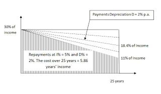
FIG 5.4 

Typically a rental will start at a cost of around 21% of income whereas a mortgage will cost more, say 30% of income.

Whereas rentals will tend to cost a similar 21% of income, and it will always cost about that same 21%, the ILS Defined Cost Mortgage will start at 30% of income and become less costly than rental about mid-way through the repayment term if D% = 4% p.a., ending at just over 11% of income for a person on average income by the 25th and final year. Rentals continue at 21% of income but the mortgagee stops paying and has a valuable asset - a home.

The above figures are based upon an agreed true interest rate for I% = 3% p.a. which is about the average rate experienced by borrowers in the UK over the period 1970 to 2002.

Interestingly, the shape of the sketch is not affected if incomes stop rising or if incomes are falling or if incomes are rising fast. As long as I% has been agreed neither the lender / investor nor the borrower needs to worry about what is going on in the economy as a whole as long as jobs are safe. And jobs will be safer on this basis because the wealth effect will not be a concern to either party - investors / borrowers.

Furthermore, if lenders base their calculations upon the mean value of I% for their economy, lenders will be lending the same amount regardless of the rate of inflation. The main variant will be the slope D%, which will vary over the short term as the market rate for funds changes. If lenders keep P% about the same, this will allow them to keep property values and collateral security fairly stable in terms of income multiples.

Doing this will also remove more of the wealth effect and that will narrow the business cycle and make jobs more secure, enabling the economy to prosper.

There is scope for collaboration between lenders and the regulators for the benefit of all parties concerned.

If the agreed value of I% were to be higher then the sketch would look like one of these:

FIG 5.5 - Effect of rising I% on the slope D% p.a.

As D% reduces as I% increases, the downwards slope reduces as shown

The actual slope is not a straight line but a curve which is steeper a first.

The chance of a lender having to pay 5% or more true interest in the UK or the USA for a ten or more year bond is small because the return on equities over the long term is less than that.

In other countries the lender will need to do some research. If the true interest rate has to be higher in order to cover the lender's costs and the cost of funds, then P% will need to be higher as well.

LESSON 5b

VARIABLE RATE ILS MORTGAGES

We need to keep both P% and 'C%' unaffected if I% rises.

This means that for every 1% added to I% we have to reduce D% by 1%.

It means that the initial value of P% (the entry cost) has to be enough to prevent I% from rising to a figure that reduces D% to an unacceptably low value.

The alternative, if that fails, is to raise the value of P% above its scheduled path, or to reduce the value of 'C%' and extend the repayment period 'N'. The risks are the same as for the current LP model. It can be done but it can be a painful experience.

LOOK CAREFULLY AT THE SAFE ENTRY COST EQUATION If both P% and C% are not changing then for every 1% that I% rises, D% has to reduce by 1% to compensate and keep P% and C% the same.

This means that we have to give D% a high enough initial value to cope with both the present value of C% but also to cope with the highest sustainable rate of I% for the national economy.

CONCLUSIONS
We want P% and C% not to alter when I% changes. Only a counter-balancing change in D% can do that. 

This means that in FIG 5.5 above the slope will become variable, but we hope it will always be downwards.

At worst, C% may have to change - or at the extreme worst P% may have to rise, just as it normally does with the current Level Payments (Y-Axis only) repayments model. But at least the amount of change in P% can be less because of the reduction made in D% and maybe C% as well.

INDEPENDENT OF THE RATE OF INFLATION / AEG% P.A.

We note that I% = r% - AEG% so those two variables, r% and AEG%, are not a major concern. They can both be high or they can both can be low or even negative, the value of D%, does not need to alter unless the difference, I% changes.

Did I explain the practical role of I% in transferring wealth from the borrower to the lender? When I% = 0% there is no wealth transfer:

FIG 5.6  - Zero true interest adds no cost to wealth / income.

Interest of 5% is added at year end and by then income has risen by 5% so the amount of income borrowed is the amount of income repaid.

 FIG 5.7  - The same again. Zero I%. This time the debt is repaid over a three year period. It makes no difference.

FIG 5.8 - Here I% = 3%. This transfers 3% of a year's income from the borrower who borrowed one year's income, to the lender.

5.9 - If 3 years' income is borrowed and I% = 3% then it adds 9% of a year's income to the debt. This is why we value costs and debts in years of income.

FIG 5.10 Here (below) I% = -3%. The mortgage is repaid over a 25 year period. The outcome is that the borrower repays 1.03 years' less income / wealth than was borrowed. 

The '% of income' figures are found by taking the cost of the payment each year as a '% of income' each year. The payment is made at year's end, after the income increase so please read the following year's income for this calculation. Add up the figures to get the Payments Total in Years of Income.

Please have a look at the money cost - it is 77% more than was borrowed!

This kind of exercise justifies us saying that money has fallen in value at AEG% p.a.

As mentioned in various pages, the meaning of wealth here is strongly linked to the definition of AEG or other index used to represent incomes.

It is not the case that the cost to a particular borrower's income is as given by the figures. It is based on an average, defined by AEG% p.a.

FIG 5.11 - Level Payments for 25 years showing how P% and C% both rise every year. In the final year C% = 100% of the outstanding wealth borrowed and gets repaid, plus the interest for that year. Remember the payment is made at year end in these illustrations.

In this sense P% always rises if the debt is being repaid. Remember the definition of a standing loan - it is that P% = constant. To repay the loan P% has to be rising.

What we are concerned about is that the increase in P% is not disturbed by a change in I%.

SETTING THE SAFETY MARGINS

The value of P% at the outset, the entry cost, depends upon the value given to 'C%' which determines how long the loan will take to repay. The value of D% has to be high enough to cope with the likely maximum sustained rise in I% above its current estimated median level. This estimated median level is used to set the entry cost value of P%.

Tests have shown that if I% rises a lot higher than the median level, and then falls a lot lower, as it has done in some nations, then the ILS Model can cope in one of two ways: varying D% correspondingly, or just leaving it close to the usual value and allowing C% to oscillate. In such extreme volatile conditions, D% and C% can go negative, but since this is temporary it does not really matter.

If the ILS Model is adopted and if governments borrow using AEG-linked or GDP-linked Bonds, then it is hard to see interest rates getting very distorted except if the currency is brought into play as a factor affecting interest rates. According to the writer this should not be a factor either if the currency pricing is done properly, and not confused by cross major currency capital flows / carry trades.

In other words, the suspicion is that these violent changes in I% will not occur if the pricing of debt and the currency are both done properly, but the reader will need to finish this course of study to be able to make a judgement on that.

Meantime, back testing using the above spreadsheet on several national sets of data has shown that:

A good way to set the entry cost (P% first year) is to write the median value of I% into the Safe Entry Cost Equation, add in D% = 4%, and C% = whatever will repay the mortgage in the specified term if those conditions were fixed.

The Spreadsheet does those calculations automatically if the total period and the value of D% are input.

NOT ALL NATIONS ARE THE SAME

Be careful not all economies are the same so please, do check this out with past data for your own economy before jumping in and setting your safe entry cost.

Typically, based on data for the UK and maybe for other developed economies where there is good competition between lenders, a mid-range value for I% could be around 2% - 3% based on past data.

And it is not likely to exceed the return on equities for too long, which seems to be less than 5% p.a. true. See Siegel's Constant and other related studies which usually come to a 7% real rate of return. As a good estimate, the true rate of return is 7% less the real rate of economic growth.

So a value of D% = 4% should cover the risk of the true rate going higher and staying higher than usual for very long. Tests have confirmed this using back-data.

This gives a safe entry cost of:

P% = 1.5% + 4% + 3% = 8.5% if we take the upper, 3% figure for I%; that is, the rate that has been average for the UK from 1970 - 2002. See FIG X below. After that rates seem to have been distorted and unsustainably low.

-------------------------

 

LESSON 5c

INGRAM'S RISK MANAGEMENT CHART - RELATIVE

The values AEG% and r% do not appear in the equation 5(i) because:

I% = r% - AEG% and it contains both variables. What matters is the difference, not the values.

If AEG% rises by 1% and r% also rises by 1% we have no change in the value of I%.

It is now possible to draw a new chart in which the Y-axis as we knew it, is abandoned and replaced with the AEG% p.a. line. Everything else remains the same except that the absolute values of r% and AEG% are not seen any more. They do not matter. They can be almost anything. Everything is relative to the AEG% line.

FIG 5.12 - Ingram's Risk Management Chart (Relative)

TRANSPORTABLE

Thus we now have a new Mortgage Model that can be transported from economy to economy and always delivers a somewhat similar entry cost equation:

P% = C% + D% + I%

If I% and D% are able to be similar then the entry cost P% will be similar at any rate of AEG% p.a. NOTE - differences creep in at extreme rates because the repayments are made at annual intervals in these spreadsheets and associated calculations.

Basically what matters is the longer term average rate of I%,which is about where the supply of mortgage finance balances the demand for it in mid-cycle conditions.

Different economies have different rates of inflation and of AEG% but the marginal rate of interest, I% still determines how fast wealth moves from borrowers to lenders.

This does not mean that they will have the same average value for I%, not exactly the same, and so the safe value for P% will vary from economy to economy, but not by too much.

For further reading on this readers are referred to the following linked pages:

LESSON 5  ANNEX - This is an extension to this lesson and should be read. Also these three links:

UNITS OF WEALTH
Siegel's Constant
Finding the Mid-Cycle Rate of Interest


LESSON 6 HAS BEEN REMOVED.

RESEARCH OPPORTUNITY
What are the implications for the developing world?

How will rising mortgage payments with possibly rising money debt be presented to the people? Can you outline a rent-to-buy contract? Don't forget people want to move house and be mobile. One contract that you could use is a fixed true rate contract which enables you to fix D% as well as I%.

If you would like a copy of Edward Ingram's spreadsheets to experiment with, let him know. They are his copyright. Please respect that. Are they for private use or business use?